Discrete Fourier Transform (DFT)
Introduction to Fourier Transform
Almost every branch of engineering and science uses Fourier methods. The words "frequency," "period," "phase," and "spectrum" are important parts of an engineer's vocabulary. The basic idea, the decomposition of signals into orthogonal trigonometric basis functions, is a natural and powerful tool which is used in a vast number of applications. We call such tools Forier methods because of the ideas of Joseph Fourier (1768-1830) and his determination to get them accepted.
When describing a digital system, the discrete time Fourier transform (DTFT) was introduced because it arises naturally as the frequency response function of a digital filter. The input-output relation
y = h * u
which relates the input, output, and unit pulse response sequences becomes
![]()
after the DTFT is applied. Thus the apparently complicated convolution operation has been transformed into multiplication.
It might seem that we should be content with studying only the DTFT, since digital signal processing must necessarily deal with discrete-time signals. Although it is true that the DTFT is our basic tool, it must be understood in context : many discrete-time signals which exist in a digital processor began life as continuous-time signals. For such signals the appropriate transform is not DTFT.
Figure TC.2.1 exhibits four separate Forier transforms, each of which is completely self-contained and appropriate to its own class of signals. There only two questions that one need ask in order to decide which transform is appropriate. Is the signal continuous in time, or discrete? And is the signal periodic? The four combinations of yes and no provide a a characterization of the appropriate transform.
If one attempts to use the wrong transform for a given signal, he or she may well succeed in getting an answer, since the four transforms have similar properties. But this usually leads to some rather unnatural signal modeling which can sometimes be deceptive. We shall see that the transforms themselves are not difficult to understand and to use. But problems such as sampling, aliasing, and the relation of the fast Fourier transform to the true Fourier transform generally involve signals from separate classes, and here one must be careful.
If you want to know more about Fourier transform, please refer to the textbooks or courses about "Signals and Systems", "Digital Signal Processing", and "Discrete Time Signal Processing".
Discrete Fourier Transform (DFT)
This transform is defined by

The inverse transformation kernel is the conjugate transpose of the forward kernel. In addition, because of the symmetry of F,
F-1 = F*T = F*
Although F and F* have complex elements of the form (a+jb), a conjugate symmetry property applies to the DFT of real-valued inputs, and as a consequence the DFT representation involves a total of only N (not 2N) elements. The conjugate symmetry is described by
y(k) = y*(N-k); k=1,2,...,(N/2)-1
so that
Re{y(k)} = Re{y(N-k)}; k=1,2,...,(N/2)-1
Im{y(k)} = -Im{y(N-k)}; k=1,2,...,(N/2)-1
Im{y(0)} = Im{y(N/2)} = 0
In the case of even N, the total number of non-redundant real-valued numbers in the DFT representation is simply N, since y(0) and y(N/2) are real-valued, and the remaining N-2 components have a total of N-2 non-redundant numbers. Therefore, for N input samples, there are exactly N unique numbers, representing the transform coefficients that have to be quantized and transmitted.
Example 1-D DFT; N=4
![]()
The DFT representation has N = 4 non-redundant numbers, -1/2, 3/2, 4 and 3. The DFT pair is shown in Figure TC.2.2. Notice that the amplitude spectrum |y(k)|, and hence the energy spectrum |y(k)|2, is symmetrical about k = N/2 = 2, except for the k = 0 term.
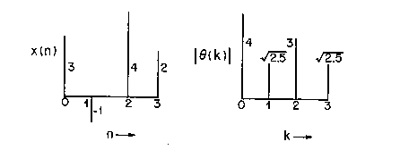
Figure TC.2.2 DFT examples: 1-D input x(n) and DFT coefficients y(k)
Implementation of the DFT and IDFT
DFT representations have two important advantages. The first is that a sine-cosine basis space is a very familiar concept. It provides a natural framework for optimizations of transform coder design with inputs where the perceptual effects of signal distortion are best understood in the frequency domain. A second advantage has to do with computation. A direct evaluation of an N-point DFT requires about N2 complex multiply-add operations; but if N is a power of 2, the Fast Fourier Transform (FFT) method needs in the order of Nlog2N operations [Elliott and Rao, 1982]. With N = 1024, the FFT is about one hundred times faster than a direct computation. The savings in computation time are approximately 32 and 18 for N = 256 and 128, respectively.
In the case of real-valued inputs, further reductions are possible by exploiting the symmetry properties of the DFT. Two N-point real sequences can be considered real and imaginary parts of a complex sequence and the 2N-point sequence can be transformed with a single transform. A simple even-odd separation recovers the real and imaginary parts of the two spectra. The procedure involves a total number of operations in the order of (Nlog2N) / 4 [Narasimha and Peterson, 1978].
The FFT algorithm can also be used to evaluate the inverse (IDFT) operation x = F*y. Indeed, by computing the DFT of the complex conjugate of y, i.e., the DFT of y*, we obtain x* = Fy*, and we obtain x by complex-conjugating the result. We finally note that FFT's usually compute a DFT that has no scaling factor and an IDFT that has a scaling by 1/N. Resulting basis vectors are orthogonal but not orthonormal.
Two-Dimensional DFT
In general, a 2-D transform requires pre-multiplication of the input with a fourth-order tensor. However, the DFT kernel
![]()
is separable and symmetric, so that
Y = FXF ; X = F*YF*
The operation can be performed with 2Nllog2N instead of 2N3 complex multiply/add operations if an FFT algorithm is applied. (Nlog2N operations for one row of X, N2log2N operations for XF, and 2N2log2N operations for FXF). Also, as in the one-dimensional case, although complex elements are involved in the matrix F, the two-dimensional representation requires only N2 numbers that have to be quantized and transmitted.